I’m an Excel fan. There’s something about a slick, well-oiled spreadsheet that floats my boat. But an Excel wizard I am not. And if you’re the same, your trusted IT support partners are here to help you.
Sure, I can cobble together some data and generate a pretty table. But it’s clunky, it takes me longer than it probably should, and I usually break something while cycling through the menus to find what I am looking for.

So, when I discovered that our very own Sales Technician now Procurement Manager, Dan Pavic, was attending a course to level up his Excel expertise, I asked him to put aside the complex formulas and share a handful of simple and effective tips that can help those of us that are a little less wizard-like and a little more fumbledore...
And sure enough, Dan shared seven tips from his Excel spell-book, to speed up your workflow and be more productive in Excel. Better yet, here’s all 7 steps in rapid action that transformed this raw (and pretty ugly) sample data into a fully functional – and presentable - spreadsheet, in less than 1 minute.
But let's take a closer look at each one of the tips demonstrated in the video.
Excel Tip #1 - Transpose
For some, this might be common knowledge but for those of you who, like me, have been manually rearranging your columns and rows around since you can remember, the transpose tool will soon have you proclaiming “Why didn’t I know about this sooner…!?”. Take a look.
Here’s our raw sample data.

In its current form, it’s pretty useless, it’s difficult to read and it would be much more helpful if it were flipped around. But instead of copying and pasting the individual rows, or worse, re-typing it out… (yes, guilty) here’s how you can use the transpose tool to flip your data around in seconds.
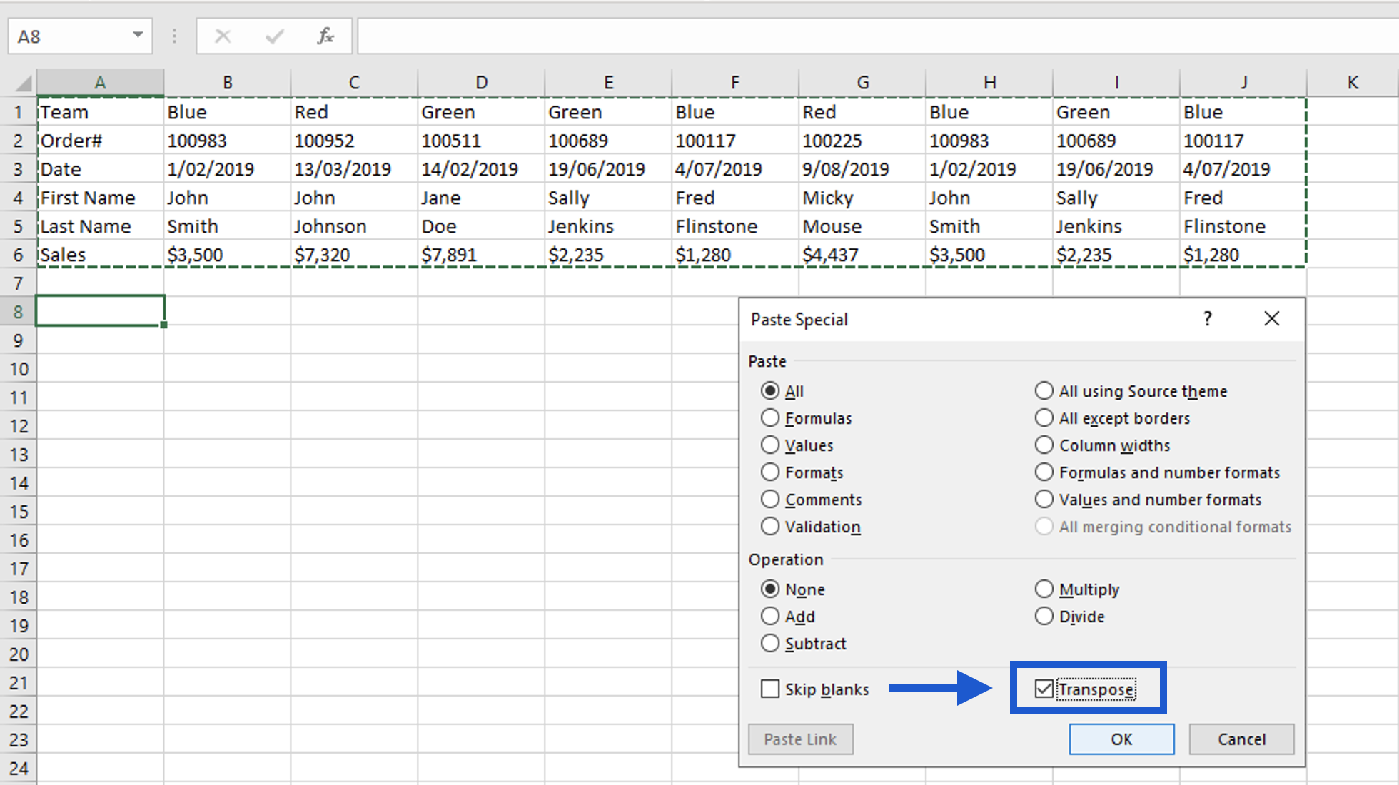
- Select your data
- Hit CTRL + C to copy your data
- Select a new cell and hit CTRL + ALT + V to bring up the ‘Paste Special’ window
- Tick the Transpose checkbox
- Click OK
Excel Tip #2 – To find what you’re looking for, just ask.
If you’re using Office 365, you can wave goodbye to the days of hunting through your menus to find an elusive tool that’s hidden in the depths of obscure icons and sub-menus.
Instead, use the ‘Tell Me’ search box (located in your ribbon) to type in whatever it is you want to do, and it will instantly retrieve the tools for you.
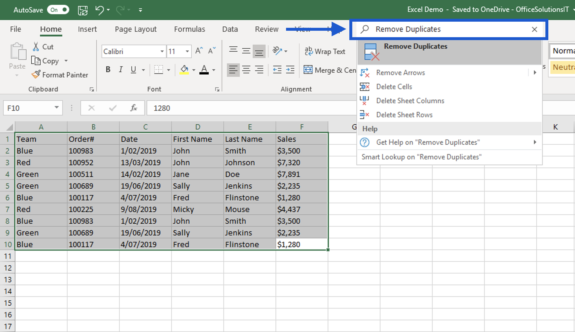
Extra tip: The ‘Tell Me’ search box isn’t restricted to Excel, it’s available in every Office 365 app. Oh, and to make accessing features even easier, you can use the keyboard shortcut ALT + Q to activate the ‘Tell me’ box directly. Here we’ll use it to quickly remove the duplicates from our data.
- Select the range of your data
- Hit ALT + Q to activate Tell Me
- Type your desired function e.g. “Remove Duplicates”, and hit enter
- Choose your settings and click OK.
Excel Tip #3 – Make your data readable. Oh and presentable.
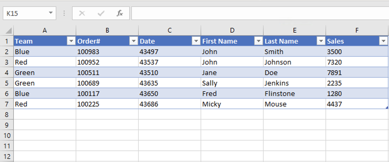
Tables are the bread and butter of Excel, they make your data easier to read and provide all sorts of handy features like built-in filters and sorting tools.
Creating a table isn’t difficult. In fact, using a keyboard shortcut to transform your raw data, so you can leverage the benefits of tables only takes a second. Give it a try, just click anywhere within your data range and hit CTRL + T.
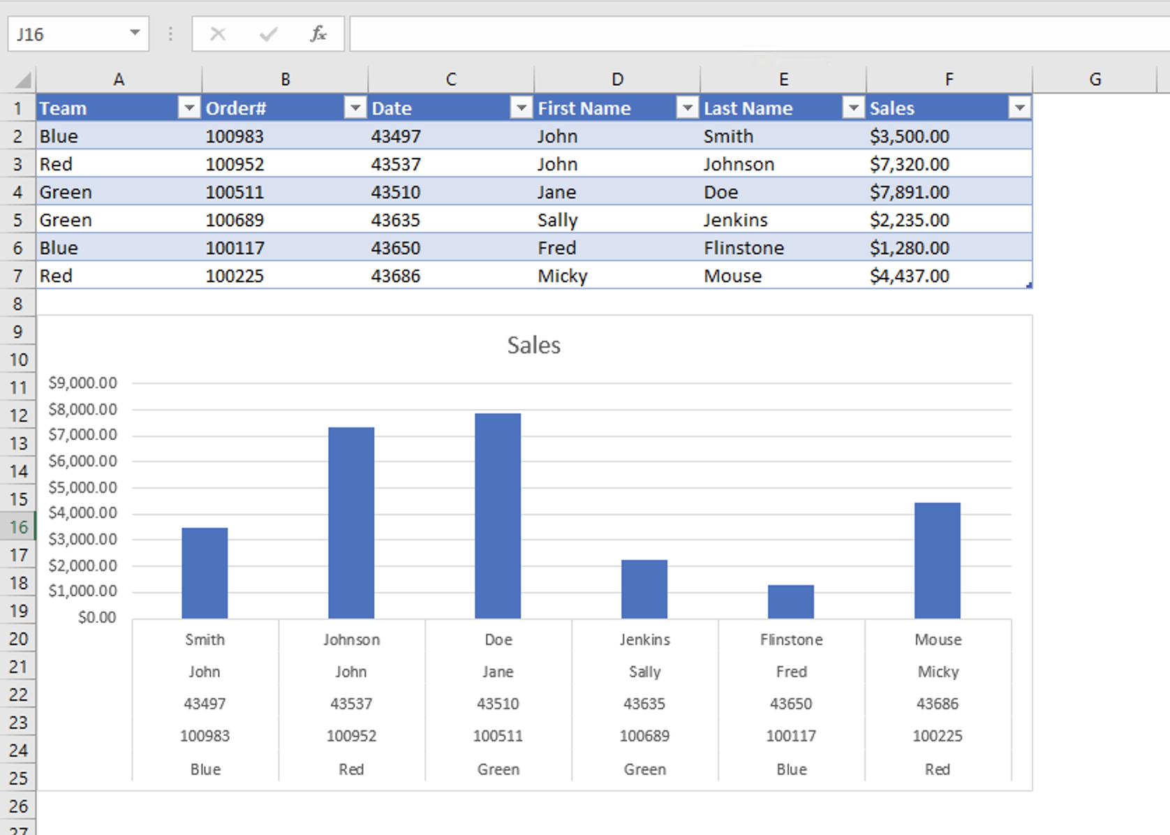
Excel Tip #4 – Make it visual
Charts help you to visualise your data, so you can quickly identify trends, scan large volumes of data and make stuff look good (yes, that’s the technical term). And much like our previous step, creating a chart from your table is only a swift shortcut away.
Simply select a cell within your table and hit ALT + F1 to instantly create a chart that you can resize and customise in a way that creates maximum impact for your audience.
Excel Tip #5 – Formula Free Totals
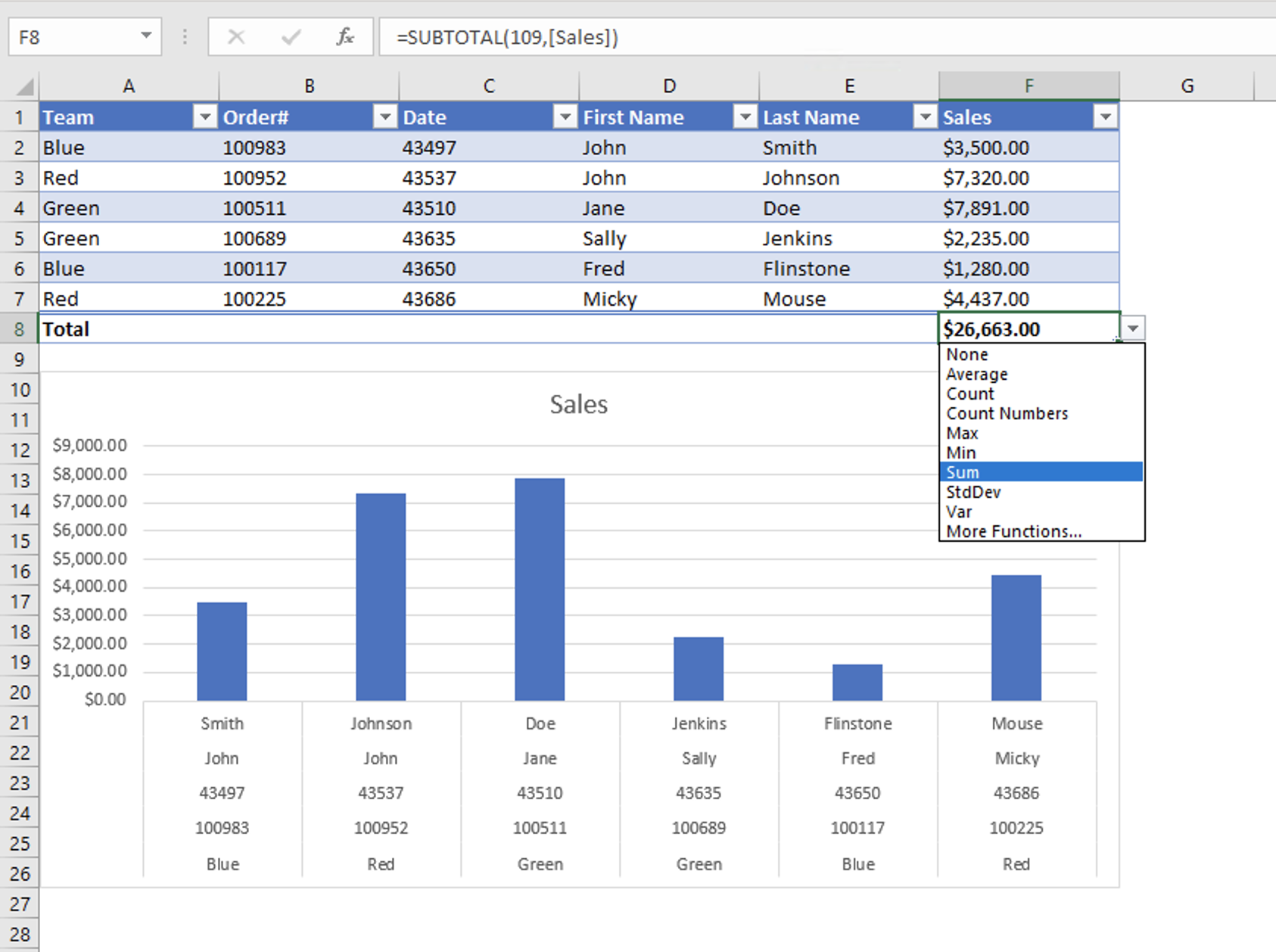
If you typically use a formula or auto-sum to calculate the total in your tables, consider using the CTRL + SHIFT + T keyboard shortcut to automatically add a total row to your table instead.
Why? Well, you don’t have to use formulas for one. And two, this flexible total gives you access to a drop-down menu to select precisely what total you want to display, such as the count, the average, minimum and maximum sales or the total sum.
Excel Tip #6 – Data Bars
Much like charts, using data bars within your tables makes your data scannable, which means it’s a lot easier for your audience to digest. Using them is simple, Oh, and they look the part too.
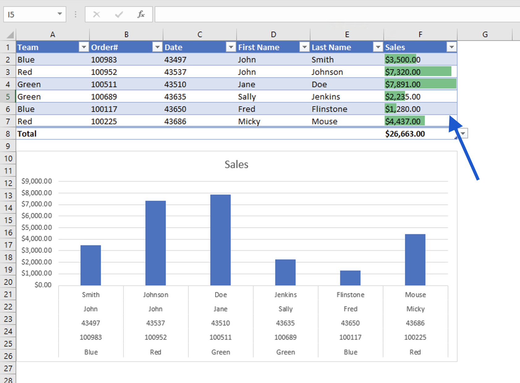
- Select your data
- Hit ALT + Q to activate Tell Me, type “Data Bars” and hit enter
- Simply click on the data bars that you’d like to insert, and Excel does the rest.
Excel Tip #7 – One-Click Slicers
A slicer is the term given to a button that allows you to instantly filter your data, so you can isolate and analyse specific areas. Take our sample table as an example, what if you wanted to isolate the sales data for each team? Well, with a slicer you can.
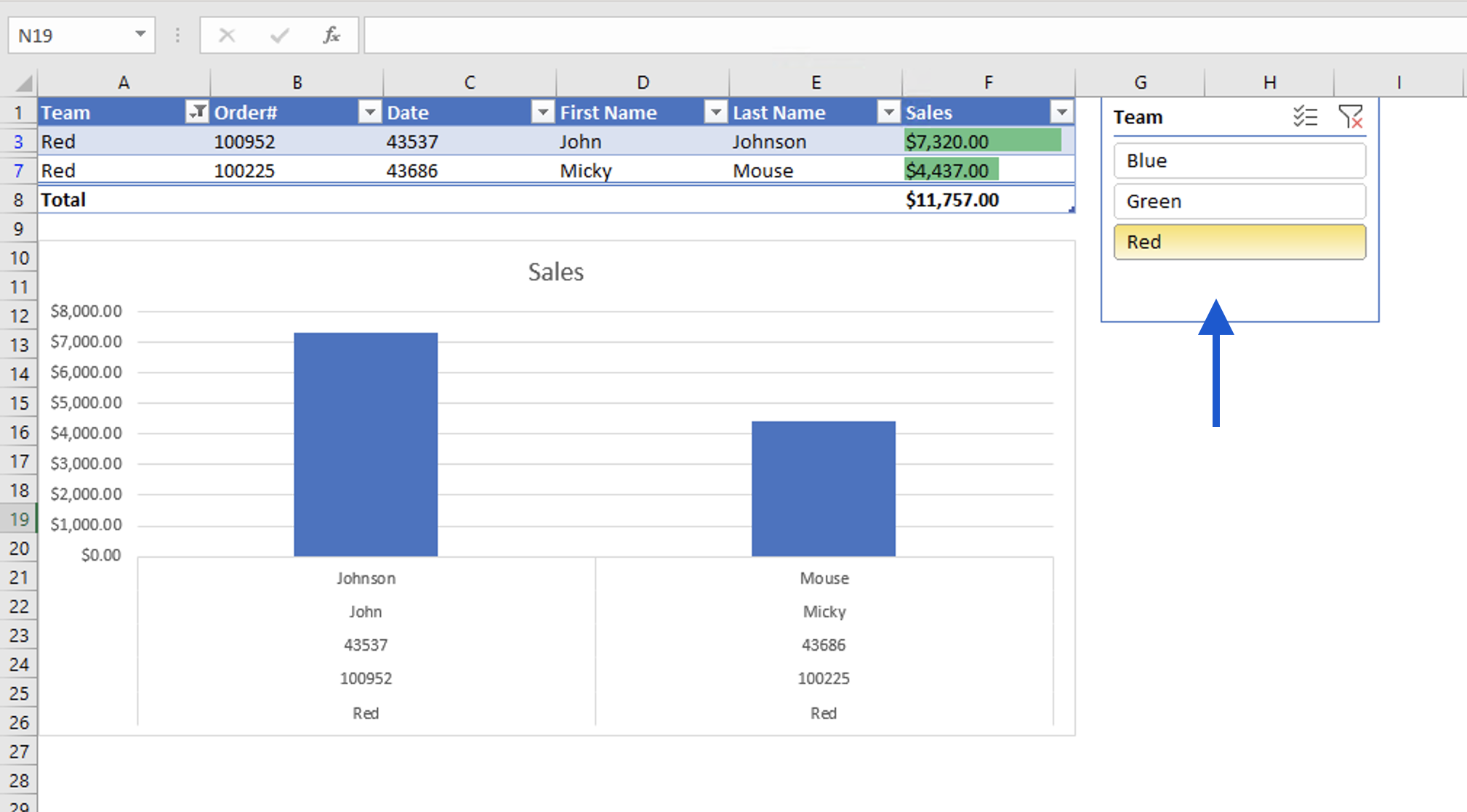
- Select any cell in your table
- Hit ALT + Q to activate Tell Me, type “slicer” and hit enter
- Choose the heading you’d like to slice your data with e.g. Team
- Click OK
Now you can click on the individual team to isolate the corresponding data. Oh, and when you do, your charts, data bars and totals that you created in steps #4, #5 & #6 will automatically update too.
Time-Saving Excel Shortcuts
Practice makes perfect with programs like Excel, and the more you learn to navigate your way around using keyboard shortcuts the more efficient you’ll become - so Dan tells me anyway.
I’ll certainly be giving these tips a go, but I’m interested, do you have a masterful Excel shortcut or tip that you use in your spreadsheets? If so, drop it in the comments. I’d appreciate it and I know fellow readers would too.
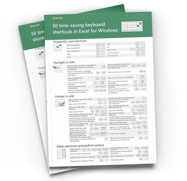
Oh, and if you’d like to get your hands on even more keyboard shortcuts, just click here to download 50 time-saving keyboard shortcuts for Excel (Windows). And don’t worry Mac users, we’ve got you covered too.
If you need further help with Excel or any of the Microsoft 365 productivity tools, your friendly neighbourhood IT support guys are willing to help.


